Probabilistic Topic Modeling
Apr 18th, 2013Probabilistic models
LSA represents topics as points in Euclidean space and documents as linear combination of topics. Probabilistic topic models differ from LSA by representing topics as distributions over words, and documents as probabilistic mixtures of topics.
Formally, given a vocabulary of $W$ words, each topic $k = 1, …, K$ has a word-distribution $\boldsymbol \varphi_k \in \Delta_W$, with $\Delta_n$ the simplex of dimension $n$, and each document $d = 1, …, D$ has a topic-distribution $\boldsymbol \theta_d \in \Delta_K$. We call $\boldsymbol \Phi$ the matrix with rows $\boldsymbol \varphi_k$ and $\boldsymbol \Theta$ the matrix with rows $\boldsymbol \theta_d$.
By estimating the model parameters $(\boldsymbol \Phi, \boldsymbol \Theta)$, we discover new knowledge about the corpus; topics are represented by the word-distributions $\boldsymbol \varphi_k$, and each document is tagged with discovered topics, which is represented by $\boldsymbol \theta_d$.
Probabilistic Latent Semantic Indexing
Probabilistic Latent Semantic Indexing (pLSI) is described as a generative process [Hofmann99], a procedure that probabilistically generates documents given the parameters of the model.
# Generative process for pLSI

procedure GenerativePLSI(document-tagging theta_d, topics phi_k):
  for document d = 1..D:
    for position i = 1..N_d in document d:
      draw a topic z_di from Discrete(theta_d)
      draw a word w_di from Discrete(phi_z_di)

  return counts n_dw = sum_i I(w_di = w)
Here is a graphical representation of the model:
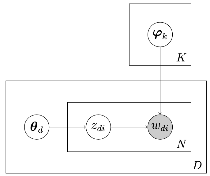 pLSI model
Parameters of the model are then learned by Bayesian inference.
Although the formulation of the model is probabilistic, [Ding08] proved the equivalence between pLSI and NMF, by showing that they both optimize the same objective function.
As they are different algorithms, they will navigate in the parameters space differently. It is possible to design an hybrid algorithm alternating between NMF and pLSI, every time jumping out of the local optimum of the other method.
Latent Dirichlet Allocation
[Blei03] extended pLSI by adding a symmetric Dirichlet prior $\text{Dir}(\alpha)$ on topic-distributions $\boldsymbol \theta_d$ of documents and derived a variational EM algorithm for the Bayesian inference. [Griffiths02a] [Griffiths02b] went further by adding a symmetric Dirichlet prior $\text{Dir}(\beta)$ on topics $\boldsymbol \varphi_k$, and derived a Gibbs sampler for the Bayesian inference. Here is the generative process of LDA.
# Generative process for LDA

procedure GenerativeLDA(document-tagging smoothing alpha, topic smoothing beta):
  for topic k = 1..K:
    draw a word-distribution phi_k from Dir(beta)
  for document d = 1..D:
    draw a topic-distribution theta_d from Dir(alpha)
    for position i = 1..N_d in document d:
      draw a topic z_di from Discrete(theta_d)
      draw a word w_di from Discrete(phi_z_di)

  return counts n_dw = sum_i I(w_di = w)
Here is a graphical representation of the model:
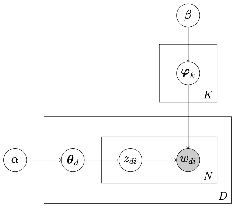 LDA model
Bayesian model can also be described graphically in plate notation which helps to understand the dependencies between random variables.
We suppose documents are generated according to this generative model and we want to estimate values for a set a parameters $(\boldsymbol \Phi, \boldsymbol \Theta)$ that can best explain the set of observations: the word counts $n_{di}$.
Theoretically, we could learn hyperparameters $\alpha$ and $\beta$ using Newton-Raphson method [Blei03]. But usually, hyperparameters are fixed heuristically to simplify the algorithm and make it converge faster. Common values are $\alpha = \frac 1 K$ and $\beta = 0.1$ [Steyvers06].